Performance Concepts

Last updated on 2024-08-31 | Edit this page

Overview

Questions

What does performance mean in programming?
How do I take advantage of optimized libraries?

Objectives

Understand that what actually goes on in the computer may be much more complex than what the user tells the computer to do.
Have a basic understanding of some of the performance issues to be aware of.
Learn that you don’t have to be an expert programmer to take advantage of advanced performance techniques, you just need to be aware of how to use libraries optimized by experts.

Conceptual View

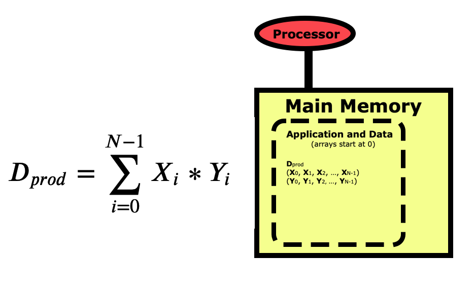
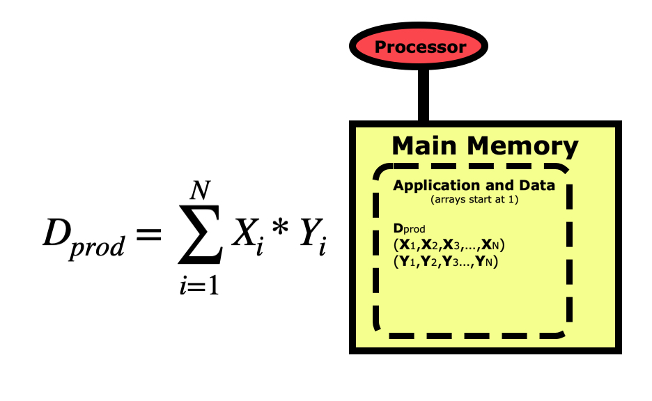
When we write a program for a computer, we view the operation from a more conceptual level. The picture below is for a simple dot product between two vectors X and Y, where the dot product D_prod is the sum of the elements of each vector multiplied together. Notice first that the indexing for arrays in Python starts at 0 and goes to N-1. This varies between languages, with C/C++ also starting at 0, while R, Matlab, and Fortran start arrays at 1 and go to N.

When we think of a computer running a program to do this calculation, we view it as starting with the variable D_prod being pulled from main memory into the processor where this sum is zeroed out. We then pull the first element of X and the first element of Y into the registers and multiply them together then summing them into D_prod. We loop through all elements of the vectors, each time pulling the X and Y element into memory, multiplying them together and summing them into D_prod. Then at the end, we push D_prod back down into main memory where the program prints the result out to the screen.

This conceptual view of what the computer is doing is all we really need to be aware of when we are starting to writing programs. But when those programs start taking too long to run on a personal computer then we need to understand what the computer is doing in more depth so we can make sure that the code is running optimally. Computers are internally quite complex, so fully understanding how code can be written in different ways to streamline the processing can be very challenging. Fortunately, not everyone needs to be able to write optimal low-level code. For most of us, we just need to understand what programming techniques in each language may cause performance problems, and understand how to take advantage of optimization libraries that experts have written for us.

The Computer’s View

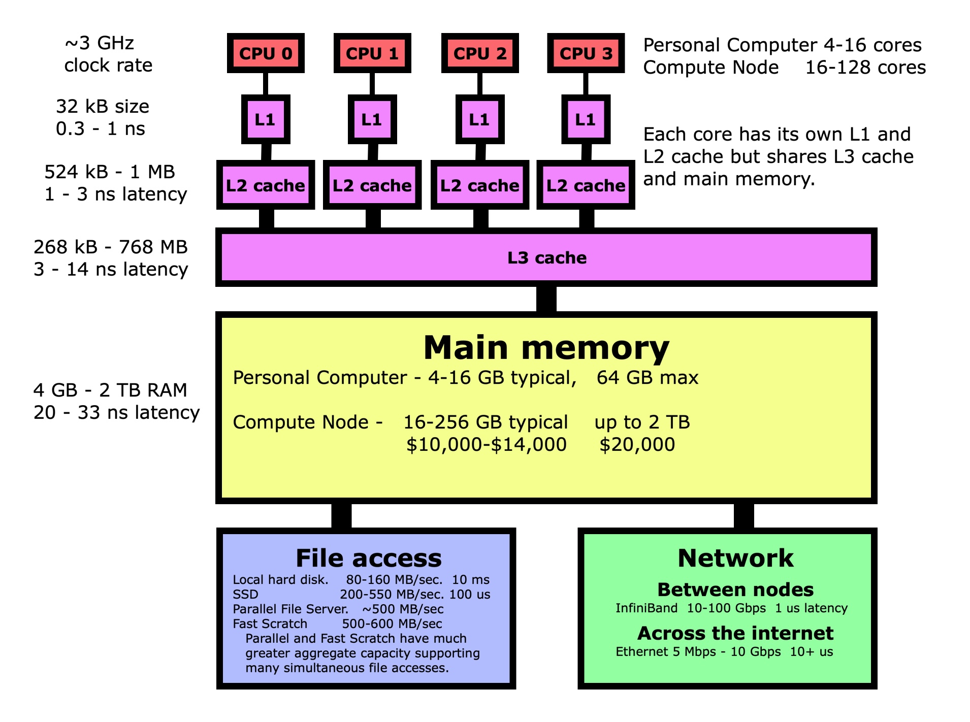
Let’s walk through the same dot product example again, but this time looking at it from the point of view of the computer rather than our conceptual view. The first thing to understand is that when you pull a variable up from main memory into the registers in a processor, what goes on behind the scene is very complicated, but fortunately for us also totally automated. Variables don’t get pulled up individually but as part of a 64-byte cache line. The variables in this cache line get promoted through several layers of increasingly fast memory known as cache layers, with a copy of the entire cache line being left behind in each layer. In this way, the most frequently used data will be more likely to be in one of the cache layers where it can be accessed more quickly. In the case of our dot product, that means loading the first element of X and its 64-byte cache line may take 10-33 ns while the next 7 only take 0.3-1 ns since those elements are now in L1 cache too.

Diagram of the memory hierarchy in a typical computer

How does this knowledge help us? Performance is more about getting data to the processor since most operations are very fast once the data is in the processor registers. If the vector is instead not stored in contiguous memory, with each variable in the next memory location, then the subsequent 7 memory loads of X and Y will take 20-33 ns each instead of 0.3-1 ns each. This means that we need to ensure that variables we are using are in contiguous memory whenever possible. There will be an exercise at the end of this section where you will measure the difference in execution time between these two cases.

Now let’s look at a simple matrix multiplication algorithm which is fairly simple to program, but may have very different performance depending on how you write the code.

Formula and diagram of a matrix multiply

Once the matrices are initialized, the code to multiply them together is fairly simple.

PYTHON

# Complete code is in code/matmult.py

N = 100
for i in range( N ):
    for j in range( N ):
        C[i][j] = 0.0
        for i in range( N ):
            C[i][j] += A[i][k] * B[k][j]

Not implemented yet.

C

// Complete code is in code/matmult.c

   N = 1000;
   for( i = 0; i < N; i++ ) {
      for( j = 0; j < N; j++ ) {
         C[i][j] = 0.0;
         for( k = 0; k < N; k++ ) {
            C[i][j] += A[i][k] * B[k][j];
         }
      }
   }

FORTRAN

! Complete code is in code/matmult.f90

   N = 1000
   DO i = 1, N
      DO j = 1, N
         C(i,j) = 0.0
         DO k = 1, N
            C( i, j ) = C( i, j ) + A( i, k ) * B( k, j )
         END DO
      END DO
   END DO

Not implemented yet.

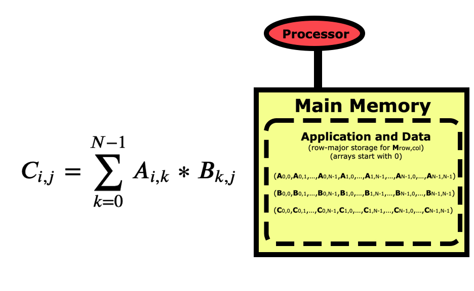
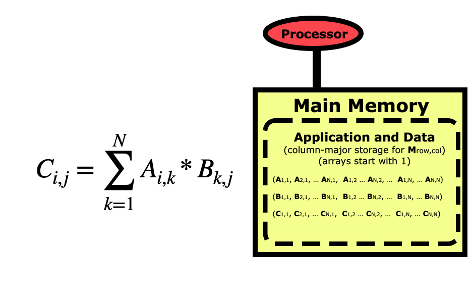
But if we are concerned about performance, we need to take a better look at this code. Python is a row-major language like C/C++, which means matrices like this are stored by rows first as in the picture above. If we look at this code from a cache-line point of view, then it looks optimal for the B matrix since when we load an element the others in the cache line will get used in the next loop iterations, but the A matrix is the opposite where elements being used next are farther apart.

But it turns out this isn’t really the way to look at performance in this case. For each element of C that we calculate, we will need N elements of A and N elements of B. So every element of A and every element of B will get re-used N times during this calculation. What is important is that when we pull each element into the L1 cache where it is the fastest to access, we want to re-use it as much as possible rather than having to pull it repeatedly from the lower caches or main memory.

An optimal approach has been developed in the past that pulls blocks of each matrix into L1 cache. This block optimization results in a much more complicated code, but also a much higher performing one. The good news is that for users like us, we don’t have to ever program it ourselves, we just need to know that it is in optimized libraries that we can call at any time. Below are some examples of how to access the low-level optimized libraries in the various languages.

PYTHON

# Complete code is in code/matmult_numpy.py

import numpy as np

N = 100
C = np.matmult( A, B )

Not implemented yet.

C

// Complete code is in code/matmult_cblas.c

#include <cblas.h>

   N = 1000;
   cblas_dgemm( CblasRowMajor, CblasNoTrans, CblasNoTrans,
                N, N, N, 1.0, *A, N, *B, N, 1.0, *C, N );

FORTRAN

! Complete code is in code/matmult_blas.f90
! gfortran -O3 -lblas -o matmult_blas matmult_blas.f90

   N = 1000
   CALL DGEMM( 'N', 'N', N, N, N, 1.0, A, N, B, N, 0.0, C, N )

Not implemented yet.

So while writing a matrix multiplication code from scratch is not difficult, using the optimized function accessible from each language is easier and guarantees the best performance. To find out how much difference there is in performance, you will need to try for yourself by measuring the execution time for a few different matrix sizes in the exercise below.

Measuring Cache Line Effects

Run the dot_product.py code several times to get an average execution time for a dot product between two vectors of 1 million elements each. Try to run them on an isolated system if possible, or through a batch queue that at least ensures the code is being run on an isolated processing core. Then run the dot_product_sparse.py code in the same manner for comparison. How much faster is the first code where the vectors are stored in contiguous memory? How much faster should it be?

Not implemented yet.

Compile and run the dot_product_c.c code several times to get an average execution time for a dot product between two vectors of 1 million elements each. Try to run them on an isolated system if possible, or through a batch queue that at least ensures the code is being run on an isolated processing core. Then compile and run the dot_product_sparse.c code in the same manner for comparison. How much faster is the first code where the vectors are stored in contiguous memory? How much faster should it be?

Compile and run the dot_product_fortran.f90 code several times to get an average execution time for a dot product between two vectors of 1 million elements each. Try to run them on an isolated system if possible, or through a batch queue that at least ensures the code is being run on an isolated processing core. Then compile and run the dot_product_fortran_sparse.f90 code in the same manner for comparison. How much faster is the first code where the vectors are stored in contiguous memory? How much faster should it be?

Not implemented yet.

Show me the solution

Is the time difference what we expected? When I ran this on a new Intel processor that did not have any other jobs running, I measured 180 milliseconds for the contiguous memory case and 1230 milliseconds for the sparse case, resulting in a 6.9 times speedup by keeping the vector in contiguous memory. Since a cache line is 64 Bytes and each element is 8 bytes, when the first element is loaded the next 7 are brought into L1 cache essentially for free since they are in contiguous memory. Therefore we expect it to take ~33 ns to load 8 elements of X, then ~33 ns to load 8 elements of Y, then only a few ns to get each element into the registers and do the computations. For the sparse vectors, it should take 8 times as long since each load will take ~33 ns. If you didn’t see an 8-times speedup, don’t worry. The cache system is actually even more complicated than this picture. The main thing to learn here is that if you take advantage of the cache line by keeping the vectors in contiguous memory, your code will run much faster.

Not implemented yet.

Is the time difference what we expected? When I ran this on a new processor that did not have any other jobs running, I measured ~16 milliseconds for the contiguous memory case and ~160 milliseconds for the sparse case, resulting in a 10 times speedup by keeping the vector in contiguous memory. Since a cache line is 64 Bytes and each element is 8 bytes, when the first element is loaded the next 7 are brought into L1 cache essentially for free since they are in contiguous memory. Therefore we expect it to take ~33 ns to load 8 elements of X, then ~33 ns to load 8 elements of Y, then only a few ns to get each element into the registers and do the computations. For the sparse vectors, it should take 8 times as long since each load will take ~33 ns. If you didn’t see an 8 times speedup exactly, don’t worry. The cache system is actually even more complicated than this picture. The main thing to learn here is that if you take advantage of the cache line by keeping the vectors in contiguous memory, your code will run much faster.

Is the time difference what we expected? When I ran this on a new processor that did not have any other jobs running, I measured ~20 milliseconds for the contiguous memory case and ~300 milliseconds for the sparse case, resulting in a 15 times speedup by keeping the vector in contiguous memory. Since a cache line is 64 Bytes and each element is 8 bytes, when the first element is loaded the next 7 are brought into L1 cache essentially for free since they are in contiguous memory. Therefore we expect it to take ~33 ns to load 8 elements of X, then ~33 ns to load 8 elements of Y, then only a few ns to get each element into the registers and do the computations. For the sparse vectors, it should take 8 times as long since each load will take ~33 ns. If you didn’t see an 8 times speedup exactly, don’t worry. The cache system is actually even more complicated than this picture. The main thing to learn here is that if you take advantage of the cache line by keeping the vectors in contiguous memory, your code will run much faster.

Not implemented yet.

Time Different Matrix Multiplication Methods

There are 2 separate codes supplied to perform the same matrix multiplication for a given matrix size, matmult.py is raw Python code and matmult_numpy.py uses the highly optimized np.matmult() function. Both programs take the matrix size as an argument, so you run using python matmult.py 100 for example to measure the performance for multiplying two 100x100 matrices. Measure the performance for each method on a small 10x10 matrix, an intermediate sized 100x100 matrix, and a large 1000x1000 matrix to see how each is affected by the optimized numpy function. You should run this through a batch scheduler if at all possible since numpy will grab any cores it can, and for a fair comparison we want to test out only the single-core performance.

Not implemented yet.

Compile and run the matmult.c and matmult_cblas.c programs to compare the times for raw C and the heavily optimized BLAS library dgemm() function. Since these use statically allocated matrices you may need to increase the stack size using ‘ulimit -s unlimited’. You may also need to use a different compile line than in the code as your BLAS library may be different on each system.

Compile and run the matmult.f90 and matmult_blas.f90 programs to compare the times for raw Fortran and the heavily optimized BLAS library DGEMM() function. Since these use statically allocated matrices you may need to increase the stack size using ‘ulimit -s unlimited’. You may also need to use a different compile line than in the code as your BLAS library may be different on each system.

Not implemented yet.

Show me the solution

For the 10x10 matrix size there are 3 matrices having 100 elements each needing 8 bytes storage, so storing all 3 matrices requires only 2.4 kB of memory. Everything fits entirely in L1 cache, so the block optimized algorithm from numpy isn’t really needed. For the 100x100 matrix size, 240 kB is needed to store all 3 matrices so they will fit entirely in L2 cache, but not L1 cache. We therefore expect a significant improvement by using the optimized np.matmult() function. For the 1000x1000 matrix size, we need 24 MB to store all 3 matrices so it will reside in L3 cache. The np.matmult() function should speed up this run by substantially more. The optimization of the numpy routine however goes far beyond just block optimizing the algorithm so that it reuses data in L1 cache though. There are also computational optimizations that allow for many multiply-add operations to occur in the same clock cycle, which is called vectorization. My measurements on a modern Intel processor more of a performance benefit for larger matrix sizes. For 1000x1000 matrices, the raw Python code was very slow at 6.5 MFlops (Million floating-point operations per second). All the optimizations in the numpy code brought the performance up to 15.4 GFlops, or a whopping 2354 times faster. Raw Python code is fairly slow in itself because it is interpreted and not compiled like C/C++/Fortran code, clearly you can do very well if you learn to use the heavily optimized library routines. C is still faster than Python, with raw C code reaching 1.6 GFlops and the optimized CBLAS DGEMM routine reaching 91 GFlops.

Not implemented yet.

For a 1000x1000 matrix I got 1.2 seconds for the raw C code when compiling with -O3 optimization. The cblas_dgemm() function took only 0.015 seconds so it was 80 times faster. Even though compiled C/C++ code is very fast, the DGEMM routine is hand-optimized for each processor.

For a 1000x1000 matrix I got 1.2 seconds for the raw Fortran code when compiling with -O3 optimization. The DGEMM() function took only 0.015 seconds so it was 80 times faster. Even though compiled C/C++/Fortran code is very fast, the DGEMM routine is hand-optimized for each processor.

Not implemented yet.

Advanced Exercise - Transpose B to cache-line optimize it

As k is incremented in the innermost loop, elements of A are being brought into cache efficiently since they are stored in contiguous memory, as we learned from the dot product example. Unfortunately, elements of B are not since they will be sparse, separated by N-1 elements each time. While in most languages we already know that we can simply use the optimized library routine speedup the code, if this wasn’t available one thing we’d consider is to transpose the B matrix so that it is stored in column-major format before doing the matrix multiplication. If you’re up for a challenge, try programming this up to see if it improves the performance compared to the original code.

Show me the solution

There are a great many levels of optimization that can be done to the matrix multiplication algorithm. Transposing B should improve the performance some. For a more complete overview of what is done in the np.matmult() algorithm and others like it, follow the link: https://en.algorithmica.org/hpc/algorithms/matmul/

Summary

When it starts taking longer to run a given program, we need to start looking beyond just whether it gives the correct answer and begin considering performance. This means we need to go beyond the conceptual view of how the program runs to look at how it makes use of the underlying hardware architecture. While this can get very complicated very quickly, most users just need to be aware of where performance bottlenecks can occur in order to avoid them. Quite often, writing optimal code just means taking advantage of highly optimized libraries that experts have written and tuned. So most of us just need to know when and where to look for these optimized routines in order to write highly optimized code.

Key Points

A computer’s view of code is more complex than a user’s view.
It’s important to understand a little about what goes on when code actually runs, but you don’t need to be able to program at that level.
Whenever possible, use code written and optimized by experts instead of writing your own version.